Reference gene stability evaluation
Introduction
Quantitative real-time PCR (qPCR) has been widely used for the quantification of target gene expression. One of the essential steps in qPCR assays is to select reference genes for normalizing the gene expression levels across the samples. In this post, we’ll use a small data set from the seawater trial of the AquaFly project. The candidate reference genes evaluated are beta-actin (actb), glyceraldehyde-3-phosphate dehydrogenase (gapdh), hypoxanthine phosphoribosyl transferase 1 (hprt1) and RNA polymerase II (rnapo2). We’ll rank the stability of reference genes based on their stability across and within the treatments as described by Kortner et al. (2011).
Getting ready
Load packages
library(tidyverse)
library(data.table)
library(summarytools)
library(cowplot)
library(PerformanceAnalytics)
library(gplots)
library(broom)
library(kableExtra)
Data import and tidy
Import data
df <- read_csv("qPCR_ref_eval.csv", col_names = T, na = "")
str(df)
Classes 'spec_tbl_df', 'tbl_df', 'tbl' and 'data.frame': 144 obs. of 8 variables:
$ Sample_ID: num 7 8 9 10 11 12 13 14 15 16 ...
$ Diet : chr "IM" "IM" "IM" "IM" ...
$ Net_pen : num 110 110 110 110 110 110 111 111 111 111 ...
$ Ref_gene : chr "gapdh" "gapdh" "gapdh" "gapdh" ...
$ PE : num 1.9 1.9 1.9 1.9 1.9 1.9 1.9 1.9 1.9 1.9 ...
$ Cq : num 18.7 18.2 18.3 18.1 18.2 ...
$ Cq_error : num 0.04 0 0.02 0.04 0.06 0.02 0.04 0.06 0.06 0.01 ...
$ Comments : chr NA NA NA NA ...
- attr(*, "spec")=
.. cols(
.. Sample_ID = col_double(),
.. Diet = col_character(),
.. Net_pen = col_double(),
.. Ref_gene = col_character(),
.. PE = col_double(),
.. Cq = col_double(),
.. Cq_error = col_double(),
.. Comments = col_character()
.. )Tidy data
# Tidy data
df <- df %>%
  arrange(Ref_gene, desc(Diet)) %>%
  mutate(Quantity = `^`(PE, -Cq)) %>% # calculate mRNA quantity
  group_by(Ref_gene, Diet)  %>%
  mutate(Mean = mean(Quantity), SD = sd(Quantity)) %>% # calculate average mRNA quantity and sd
  ungroup() %>%
  group_by(Ref_gene) %>%
  mutate(Quantity_std = scale(Quantity), # standardize mRNA quantity of each reference gene
         Quantity_nm = Quantity / Quantity[1]) # normalize mRNA quantity to the first sample

# Convert Sample_ID and Net_pen to character variables
df <- within(df, {
  Sample_ID <- as.character(Sample_ID)
  Net_pen <- as.character(Net_pen)
})

# Convert Diet and Sample_ID to factors, specifying the desired orders for plotting
df$Diet <- factor(df$Diet, levels = c("REF", "IM"))
df$Sample_ID <- factor(df$Sample_ID, levels = unique(df$Sample_ID))
Exploratory data analysis (EDA)
Before we proceed to reference gene stability evaluation, we can do some exploratory data analyses, an essential step in the data analysis pipeline.
EDA by descriptive statistics
As the package providing descriptive statistics summarize data by columns, we’ll convert the dataframe from the “long” to “wide” format.
# Convert dataframe to a data.table object
dt <- as.data.table(df)

# Transform data.table from long to wide
df_wider <- dcast(dt, Sample_ID + Diet + Net_pen ~ Ref_gene, value.var = colnames(dt)[5:13])
Get descriptive statistics.
print(dfSummary(df_wider, valid.col = FALSE, graph.magnif = 0.75), max.tbl.height = 500, method = "render")Data Frame Summary
df_widerDimensions: 36 x 39
Duplicates: 0
| Variable | Stats / Values | Freqs (% of Valid) | Graph | Missing | ||||||||||||||||||||||||||||||||||||||||||||
|---|---|---|---|---|---|---|---|---|---|---|---|---|---|---|---|---|---|---|---|---|---|---|---|---|---|---|---|---|---|---|---|---|---|---|---|---|---|---|---|---|---|---|---|---|---|---|---|---|
| Sample_ID [factor] | 1. 13 2. 14 3. 15 4. 16 5. 17 6. 18 7. 25 8. 26 9. 27 10. 28 [ 26 others ] |
|  | 0 (0%) | ||||||||||||||||||||||||||||||||||||||||||||
| Diet [factor] | 1. REF 2. IM |
|  | 0 (0%) | ||||||||||||||||||||||||||||||||||||||||||||
| Net_pen [character] | 1. 101 2. 104 3. 105 4. 106 5. 110 6. 111 |
|  | 0 (0%) | ||||||||||||||||||||||||||||||||||||||||||||
| PE_actb [numeric] | 1 distinct value |
|  | 0 (0%) | ||||||||||||||||||||||||||||||||||||||||||||
| PE_gapdh [numeric] | 1 distinct value |
| | 0 (0%) | ||||||||||||||||||||||||||||||||||||||||||||
| PE_hprt1 [numeric] | 1 distinct value |
| | 0 (0%) | ||||||||||||||||||||||||||||||||||||||||||||
| PE_rnapo2 [numeric] | 1 distinct value |
| | 0 (0%) | ||||||||||||||||||||||||||||||||||||||||||||
| Cq_actb [numeric] | Mean (sd) : 14.7 (0.2) min < med < max: 14.4 < 14.7 < 15.3 IQR (CV) : 0.3 (0) | 30 distinct values |  | 0 (0%) | ||||||||||||||||||||||||||||||||||||||||||||
| Cq_gapdh [numeric] | Mean (sd) : 18.1 (0.2) min < med < max: 17.8 < 18.1 < 18.7 IQR (CV) : 0.3 (0) | 29 distinct values |  | 0 (0%) | ||||||||||||||||||||||||||||||||||||||||||||
| Cq_hprt1 [numeric] | Mean (sd) : 22.2 (0.3) min < med < max: 21.6 < 22.2 < 23.1 IQR (CV) : 0.3 (0) | 30 distinct values |  | 0 (0%) | ||||||||||||||||||||||||||||||||||||||||||||
| Cq_rnapo2 [numeric] | Mean (sd) : 24 (0.2) min < med < max: 23.6 < 23.9 < 24.7 IQR (CV) : 0.3 (0) | 28 distinct values |  | 0 (0%) | ||||||||||||||||||||||||||||||||||||||||||||
| Cq_error_actb [numeric] | Mean (sd) : 0 (0) min < med < max: 0 < 0 < 0.1 IQR (CV) : 0 (0.7) | 11 distinct values |  | 0 (0%) | ||||||||||||||||||||||||||||||||||||||||||||
| Cq_error_gapdh [numeric] | Mean (sd) : 0 (0) min < med < max: 0 < 0 < 0.2 IQR (CV) : 0 (0.9) | 11 distinct values |  | 0 (0%) | ||||||||||||||||||||||||||||||||||||||||||||
| Cq_error_hprt1 [numeric] | Mean (sd) : 0.1 (0.1) min < med < max: 0 < 0.1 < 0.2 IQR (CV) : 0.1 (0.7) | 17 distinct values |  | 0 (0%) | ||||||||||||||||||||||||||||||||||||||||||||
| Cq_error_rnapo2 [numeric] | Mean (sd) : 0.1 (0.1) min < med < max: 0 < 0.1 < 0.2 IQR (CV) : 0.1 (0.8) | 15 distinct values |  | 0 (0%) | ||||||||||||||||||||||||||||||||||||||||||||
| Comments_actb [character] | 1. Calibrated_Cq_from_run_2 |
| | 35 (97.22%) | ||||||||||||||||||||||||||||||||||||||||||||
| Comments_gapdh [character] | 1. Calibrated_Cq_from_run_2 |
| | 35 (97.22%) | ||||||||||||||||||||||||||||||||||||||||||||
| Comments_hprt1 [character] | 1. Calibrated_Cq_from_run_2 |
| | 35 (97.22%) | ||||||||||||||||||||||||||||||||||||||||||||
| Comments_rnapo2 [character] | 1. Calibrated_Cq_from_run_2 |
| | 35 (97.22%) | ||||||||||||||||||||||||||||||||||||||||||||
| Quantity_actb [numeric] | Mean (sd) : 0 (0) min < med < max: 0 < 0 < 0 IQR (CV) : 0 (0.1) | 30 distinct values |  | 0 (0%) | ||||||||||||||||||||||||||||||||||||||||||||
| Quantity_gapdh [numeric] | Mean (sd) : 0 (0) min < med < max: 0 < 0 < 0 IQR (CV) : 0 (0.1) | 29 distinct values |  | 0 (0%) | ||||||||||||||||||||||||||||||||||||||||||||
| Quantity_hprt1 [numeric] | Mean (sd) : 0 (0) min < med < max: 0 < 0 < 0 IQR (CV) : 0 (0.2) | 30 distinct values |  | 0 (0%) | ||||||||||||||||||||||||||||||||||||||||||||
| Quantity_rnapo2 [numeric] | Mean (sd) : 0 (0) min < med < max: 0 < 0 < 0 IQR (CV) : 0 (0.1) | 28 distinct values |  | 0 (0%) | ||||||||||||||||||||||||||||||||||||||||||||
| Mean_actb [numeric] | Min : 0 Mean : 0 Max : 0 |
|  | 0 (0%) | ||||||||||||||||||||||||||||||||||||||||||||
| Mean_gapdh [numeric] | Min : 0 Mean : 0 Max : 0 |
| | 0 (0%) | ||||||||||||||||||||||||||||||||||||||||||||
| Mean_hprt1 [numeric] | Min : 0 Mean : 0 Max : 0 |
| | 0 (0%) | ||||||||||||||||||||||||||||||||||||||||||||
| Mean_rnapo2 [numeric] | Min : 0 Mean : 0 Max : 0 |
| | 0 (0%) | ||||||||||||||||||||||||||||||||||||||||||||
| SD_actb [numeric] | Min : 0 Mean : 0 Max : 0 |
| | 0 (0%) | ||||||||||||||||||||||||||||||||||||||||||||
| SD_gapdh [numeric] | Min : 0 Mean : 0 Max : 0 |
| | 0 (0%) | ||||||||||||||||||||||||||||||||||||||||||||
| SD_hprt1 [numeric] | Min : 0 Mean : 0 Max : 0 |
| | 0 (0%) | ||||||||||||||||||||||||||||||||||||||||||||
| SD_rnapo2 [numeric] | Min : 0 Mean : 0 Max : 0 |
| | 0 (0%) | ||||||||||||||||||||||||||||||||||||||||||||
| Quantity_std_actb [numeric] | Mean (sd) : 0 (1) min < med < max: -2.4 < -0.1 < 1.6 IQR (CV) : 1.6 (2798353166521473) | 30 distinct values |  | 0 (0%) | ||||||||||||||||||||||||||||||||||||||||||||
| Quantity_std_gapdh [numeric] | Mean (sd) : 0 (1) min < med < max: -2.5 < -0.1 < 1.6 IQR (CV) : 1.5 (3578176847952066) | 29 distinct values |  | 0 (0%) | ||||||||||||||||||||||||||||||||||||||||||||
| Quantity_std_hprt1 [numeric] | Mean (sd) : 0 (1) min < med < max: -2.3 < 0 < 2.4 IQR (CV) : 1.1 (5862571499920934) | 30 distinct values |  | 0 (0%) | ||||||||||||||||||||||||||||||||||||||||||||
| Quantity_std_rnapo2 [numeric] | Mean (sd) : 0 (1) min < med < max: -2.9 < 0.1 < 1.9 IQR (CV) : 1.4 (1897607103291092) | 28 distinct values |  | 0 (0%) | ||||||||||||||||||||||||||||||||||||||||||||
| Quantity_nm_actb [numeric] | Mean (sd) : 1.1 (0.1) min < med < max: 0.8 < 1.1 < 1.4 IQR (CV) : 0.2 (0.1) | 30 distinct values |  | 0 (0%) | ||||||||||||||||||||||||||||||||||||||||||||
| Quantity_nm_gapdh [numeric] | Mean (sd) : 1.1 (0.1) min < med < max: 0.7 < 1.1 < 1.3 IQR (CV) : 0.2 (0.1) | 29 distinct values |  | 0 (0%) | ||||||||||||||||||||||||||||||||||||||||||||
| Quantity_nm_hprt1 [numeric] | Mean (sd) : 0.9 (0.2) min < med < max: 0.5 < 0.9 < 1.4 IQR (CV) : 0.2 (0.2) | 30 distinct values |  | 0 (0%) | ||||||||||||||||||||||||||||||||||||||||||||
| Quantity_nm_rnapo2 [numeric] | Mean (sd) : 1 (0.1) min < med < max: 0.6 < 1 < 1.2 IQR (CV) : 0.2 (0.1) | 28 distinct values |  | 0 (0%) | ||||||||||||||||||||||||||||||||||||||||||||
EDA by visualization
Dot chart
# Make a dataframe containing the grand mean of mRNA quantity
gm <- df %>%
group_by(Ref_gene) %>%
summarize(gmean = mean(Quantity))
# Make dot charts showing individual expression profile
p1 <- df %>%
ggplot(aes(x = Sample_ID, y = Quantity, group = 1)) +
geom_point(aes(color = Diet)) +
geom_line() +
facet_wrap(~ Ref_gene, ncol = 1, scales = "free_y") +
labs(y = "mRNA quantity", tag = "A") +
scale_y_continuous(labels = scales::scientific) +
geom_hline(aes(yintercept = gmean), gm, color = "blue") + # The blue line shows the grand mean.
theme_bw()
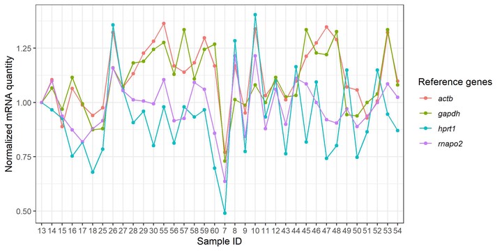
# Make dot charts showing normalized expression levels
p2 <- df %>%
ggplot(aes(x = Sample_ID, y = Quantity_nm, color = Ref_gene)) +
geom_point() +
geom_line(aes(group = Ref_gene)) +
labs(y = "normalized mRNA quantity", tag = "B") +
theme_bw() +
scale_fill_brewer(palette = "Dark2")
# Combine the plots
plot_grid(p1, p2, ncol = 1, align = "v", rel_heights = c(3, 2))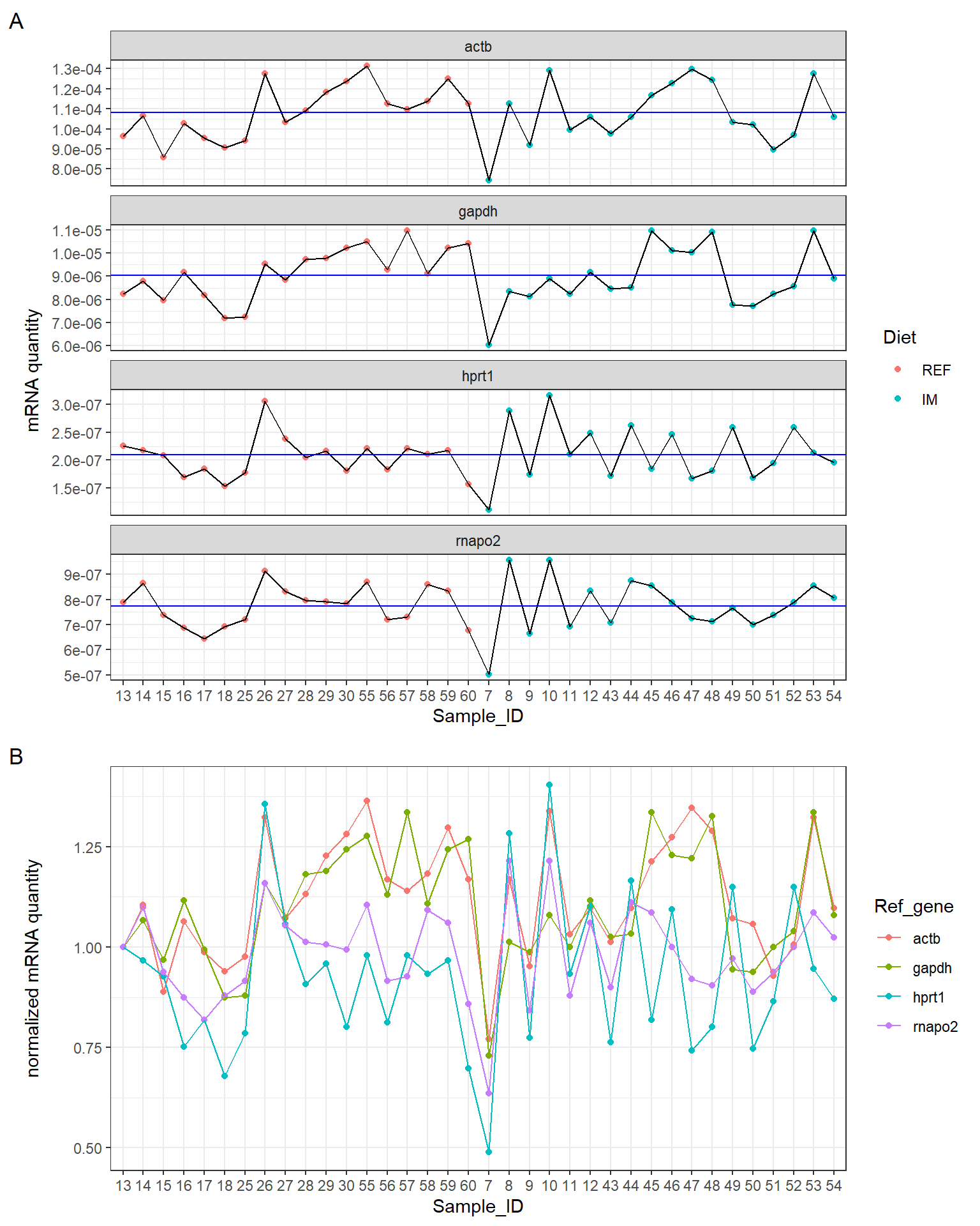
Boxplot
# Convert "Sample_ID"" to character, otherwise ggrepel won't work properly
df$Sample_ID <- as.character(df$Sample_ID)

# Define a function for identifying outliers
is_outlier <- function(x) {
  x < quantile(x, 0.25) - 1.5 * IQR(x) | x > quantile(x, 0.75) + 1.5 * IQR(x)
}

# Make plots using standardized mRNA quantity
df %>%
  group_by(Ref_gene) %>%
  mutate(outlier = is_outlier(Quantity_std)) %>%
  ggplot(aes(x = Ref_gene, y = Quantity_std, label = ifelse(outlier, Sample_ID, NA))) +
  geom_violin(trim = FALSE) +
  geom_boxplot(outlier.shape = NA, width = 0.5) +
  geom_point(aes(fill = Diet, colour = Diet), size = 3, shape = 21, position = position_jitterdodge(0.2)) +
  ggrepel::geom_text_repel(aes(colour = Diet), position = position_jitterdodge(0.2)) + # label outliers
  ylab("standardized mRNA quantity") +
  theme_cowplot() +
  guides(colour = F)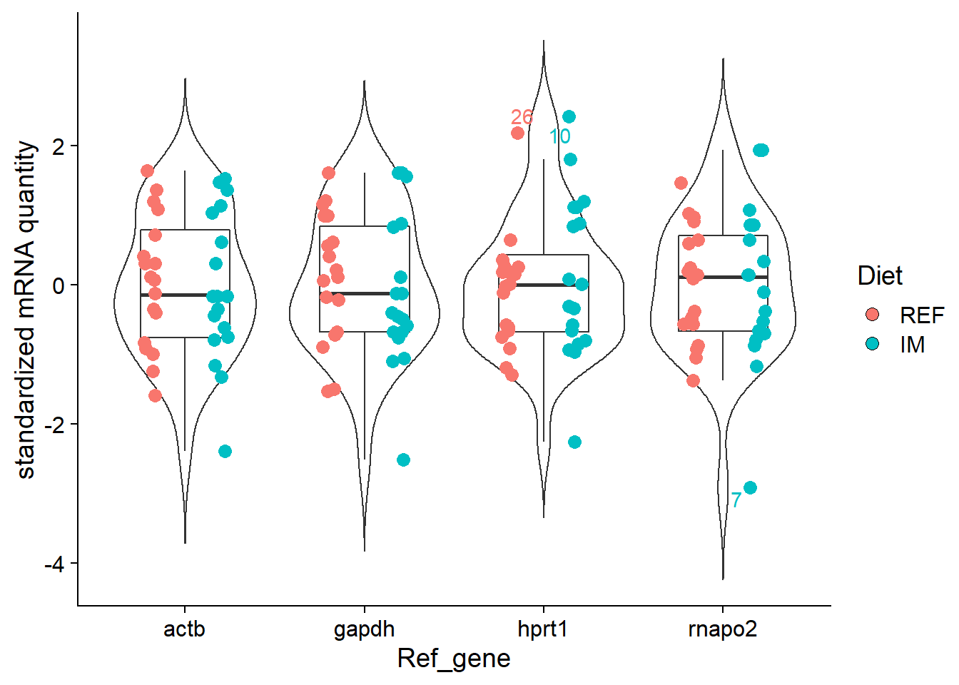
Bar plot
df %>%
  ggplot(aes(x = Diet, y =  Mean, fill = Diet)) +
  geom_bar(stat = "identity", position = position_dodge(), colour = "black") +
  geom_errorbar(aes(ymin = Mean, ymax = Mean + SD), size = 0.3, width = 0.2) + # add error bar (sd)
  facet_wrap(~ Ref_gene, nrow = 1, scales = "free_y") +
  scale_y_continuous(limits = c(0, NA), expand = expand_scale(mult = c(0, 0.1))) +
  ylab("mRNA quantity") +
  theme_cowplot()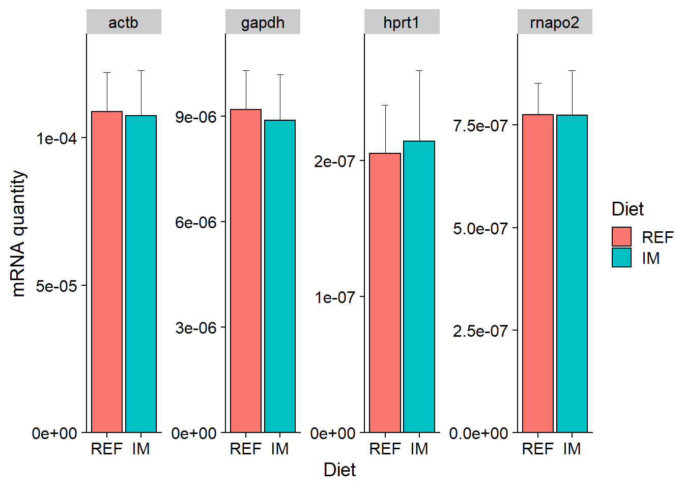
Correlation
# Subset dataframe and convert to the wide format
df1 <- df %>%
  select(Sample_ID, Ref_gene, Quantity) %>%
  spread(key = "Ref_gene", value = "Quantity")

# Make a correlation chart
chart.Correlation(df1[2:ncol(df1)], histogram = TRUE, pch = 19)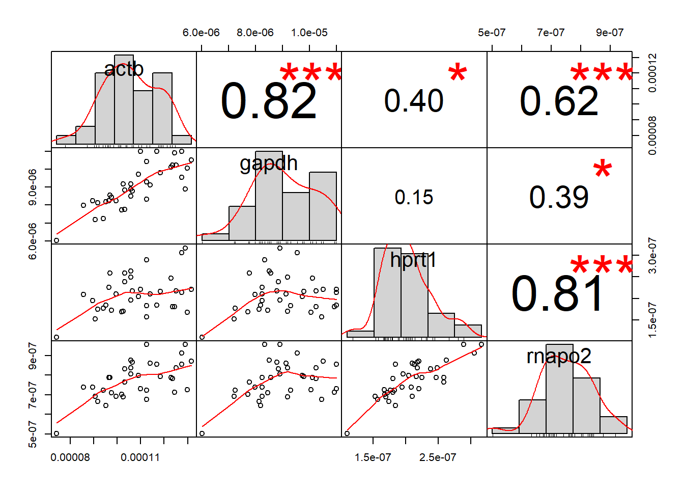
heatmap
# Make a numeric metrix for plotting heatmap
mat <- as.matrix(df1[2:ncol(df1)]) %>%
  `row.names<-`(df1[[1]]) # Sample_ID as rownames

# Define color scheme
col <- colorRampPalette(c("blue", "white", "red"))(25)

# Make heatmap
heatmap.2(mat,
          Rowv = TRUE,
          Colv = TRUE,
          distfun = function(x) dist(x,method = 'euclidean'),
          hclustfun = function(x) hclust(x,method = 'ward.D2'),
          ylab = "Sample ID",
          dendrogram = "column",
          density.info = "none",
          scale = "column",
          trace = "none",
          cexCol = 1,
          cexRow = 0.5,
          srtCol = 45,
col = col) 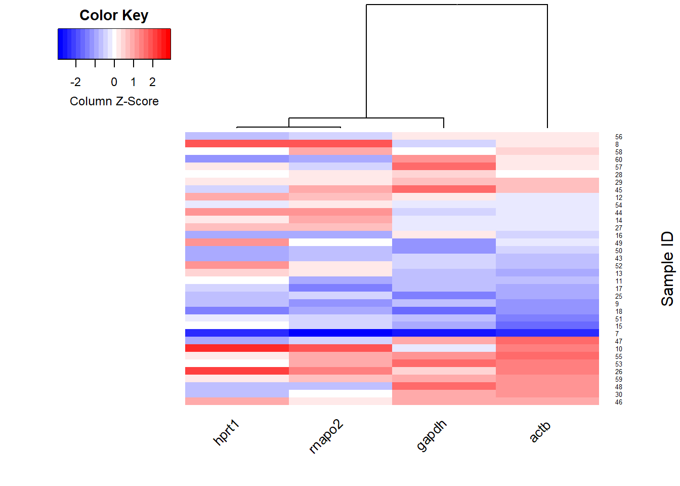
Evaluation of reference gene stability
Ranks by F-statistic
The F-statistic is a measurement of reference gene stability across experimental treatments. The smaller the F-statistic is, the better.
F_stat <- df %>%
  group_by(Ref_gene) %>%
  do(tidy(aov(Quantity ~ Diet, data = .))) %>% # run ANOVA and tidy statistical outputs
  na.omit() %>%
  select(Ref_gene, statistic) %>%
  rename(Quantity_F = statistic) %>%
  as.data.frame() %>%
  mutate(F_rank = dense_rank(Quantity_F)) %>% # rank reference genes by F statistic
  arrange(Ref_gene)
Ranks by coefficient of variance (cv)
Coefficient of variance (cv) is a measurement of overall stability of reference genes across all the samples. The smaller the CV is, the better.
cv <- df %>%
  group_by(Ref_gene) %>%
  summarize(Cq_max = max(Cq),
            Cq_min = min(Cq),
            Cq_range = max(Cq) - min(Cq),
            Quantity_mean = mean(Quantity),
            Quantity_SD = sd(Quantity),
            Quantity_CV = 100 * Quantity_SD / Quantity_mean) %>%
  mutate(CV_rank = dense_rank(Quantity_CV)) %>% # rank reference genes by CV
  arrange(Ref_gene)
Summary of ranks
# Merge tables
smr <- full_join(F_stat, cv, by = "Ref_gene")

# Format digits
smr$Quantity_mean <- formatC(smr$Quantity_mean, format = "e", digits = 1)
smr$Quantity_SD <- formatC(smr$Quantity_SD, format = "e", digits = 2)

# Format table
kable(smr, format = "html", digits = 2, align = "l") %>%
kable_styling(bootstrap_options = c("striped", "hover"), font_size = 14, position = "left")| Ref_gene | Quantity_F | F_rank | Cq_max | Cq_min | Cq_range | Quantity_mean | Quantity_SD | Quantity_CV | CV_rank |
|---|---|---|---|---|---|---|---|---|---|
| actb | 0.07 | 2 | 15.32 | 14.40 | 0.92 | 1.1e-04 | 1.42e-05 | 13.08 | 2 |
| gapdh | 0.58 | 4 | 18.73 | 17.79 | 0.94 | 9.0e-06 | 1.21e-06 | 13.33 | 3 |
| hprt1 | 0.37 | 3 | 23.11 | 21.59 | 1.52 | 2.1e-07 | 4.40e-08 | 21.00 | 4 |
| rnapo2 | 0.00 | 1 | 24.68 | 23.58 | 1.10 | 7.7e-07 | 9.37e-08 | 12.10 | 1 |
Since in most cases we’re interested in comparing the target gene expression levels across different experimental treatments, we want to select reference genes with small between-group variations, i.e., small F-statistic. Secondly, we also disire small variations in the expression level of reference genes, i.e., small coefficient of variance. Based on these two criteria, we rank the candidate reference genes as: rnapo2 > actb > gapdh > hprt1. Now that we have the ranks, the secltion of reference genes for normalization should be further evaluated based on the effect size and the variation of target genes. For more discussions on the selection of reference genes, check the paper by Kortner et al. (2011).
References
Kortner, Trond M, Elin C Valen, Henrik Kortner, Inderjit S Marjara, Åshild Krogdahl, and Anne Marie Bakke. 2011. “Candidate Reference Genes for Quantitative Real-Time Pcr (qPCR) Assays During Development of a Diet-Related Enteropathy in Atlantic Salmon (Salmo Salar L.) and the Potential Pitfalls of Uncritical Use of Normalization Software Tools.” Aquaculture 318 (3-4): 355–63.
Session info
R version 3.6.1 (2019-07-05)
Platform: x86_64-w64-mingw32/x64 (64-bit)
Running under: Windows 10 x64 (build 18362)

Matrix products: default

locale:
[1] LC_COLLATE=English_United States.1252
[2] LC_CTYPE=English_United States.1252
[3] LC_MONETARY=English_United States.1252
[4] LC_NUMERIC=C
[5] LC_TIME=English_United States.1252

attached base packages:
[1] stats     graphics  grDevices utils     datasets  methods   base

other attached packages:
 [1] kableExtra_1.1.0           broom_0.5.2
 [3] gplots_3.0.1.1             PerformanceAnalytics_1.5.3
 [5] xts_0.11-2                 zoo_1.8-6
 [7] cowplot_1.0.0              data.table_1.12.2
 [9] forcats_0.4.0              stringr_1.4.0
[11] dplyr_0.8.3                purrr_0.3.2
[13] readr_1.3.1                tidyr_0.8.3
[15] tibble_2.1.3               ggplot2_3.2.1
[17] tidyverse_1.2.1            summarytools_0.9.3
[19] knitr_1.24

loaded via a namespace (and not attached):
 [1] httr_1.4.1         jsonlite_1.6       viridisLite_0.3.0
 [4] modelr_0.1.5       gtools_3.8.1       assertthat_0.2.1
 [7] highr_0.8          pander_0.6.3       cellranger_1.1.0
[10] yaml_2.2.0         ggrepel_0.8.1      pillar_1.4.2
[13] backports_1.1.5    lattice_0.20-38    glue_1.3.1
[16] quadprog_1.5-7     digest_0.6.21      pryr_0.1.4
[19] checkmate_1.9.4    rvest_0.3.4        colorspace_1.4-1
[22] htmltools_0.3.6    plyr_1.8.4         pkgconfig_2.0.3
[25] haven_2.1.1        magick_2.1         bookdown_0.12
[28] scales_1.0.0       webshot_0.5.1      gdata_2.18.0
[31] generics_0.0.2     withr_2.1.2        lazyeval_0.2.2
[34] cli_1.1.0          magrittr_1.5       crayon_1.3.4
[37] readxl_1.3.1       evaluate_0.14      nlme_3.1-140
[40] xml2_1.2.2         rapportools_1.0    blogdown_0.15
[43] tools_3.6.1        hms_0.5.0          matrixStats_0.54.0
[46] munsell_0.5.0      compiler_3.6.1     caTools_1.17.1.2
[49] rlang_0.4.0        grid_3.6.1         RCurl_1.95-4.12
[52] rstudioapi_0.10    bitops_1.0-6       tcltk_3.6.1
[55] labeling_0.3       rmarkdown_1.14     gtable_0.3.0
[58] codetools_0.2-16   R6_2.4.0           lubridate_1.7.4
[61] zeallot_0.1.0      KernSmooth_2.23-15 stringi_1.4.3
[64] Rcpp_1.0.2         vctrs_0.2.0        tidyselect_0.2.5
[67] xfun_0.8